The Schrödinger Equation

Hydrogen

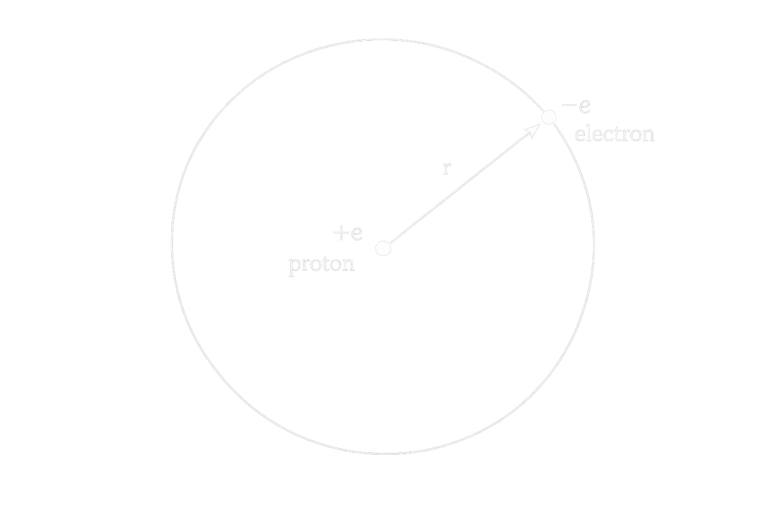
The hydrogen atom is the cleanest realistic quantum system in which the machinery of spherical coordinates becomes physically meaningful. We have a proton of charge $ +e $, which we place at the origin, and a much lighter electron of charge $ -e $ moving around it.

From Coulomb's law, the potential energy of the electron is

$$ V(r) = - \frac{e^2}{4\pi\epsilon_0} \frac{1}{r} $$

Substituting this into the radial part of the Schrödinger equation gives

$$ -\frac{\hbar^2}{2m_e}\frac{d^2u}{dr^2} + \left( -\frac{e^2}{4\pi\epsilon_0 r} + \frac{\hbar^2}{2m_e}\frac{\ell(\ell+1)}{r^2} \right)u = Eu $$

The Coulomb potential is attractive; it pulls the electron inward toward the proton. The second term is the centrifugal term, which becomes important near the origin when $ \ell>0 $. Thus the effective potential is not merely the Coulomb potential, but the Coulomb potential modified by angular momentum.

The Radial Wave Function

For bound states, the energy is negative. It is therefore useful to define

$$ \kappa \equiv \frac{\sqrt{-2m_eE}}{\hbar} $$

Dividing the radial equation by $ E $, we obtain

$$ \frac{1}{\kappa^2}\frac{d^2u}{dr^2} = \left( 1 - \frac{m_ee^2}{2\pi\epsilon_0\hbar^2\kappa} \frac{1}{\kappa r} + \frac{\ell(\ell+1)}{(\kappa r)^2} \right)u $$

This suggests introducing the dimensionless variables

$$ \rho=\kappa r, \qquad \rho_0= \frac{m_ee^2}{2\pi\epsilon_0\hbar^2\kappa} $$

The radial equation then becomes

$$ \frac{d^2u}{d\rho^2} = \left( 1 - \frac{\rho_0}{\rho} + \frac{\ell(\ell+1)}{\rho^2} \right)u $$

To understand the structure of the solutions, first examine the large-$ \rho $ limit. As $ \rho\to\infty $, the constant term dominates, and the equation becomes approximately

$$ \frac{d^2u}{d\rho^2}=u $$

Hence

$$ u(\rho)=Ae^{-\rho}+Be^{\rho} $$

The growing exponential is not normalizable, so we must set $ B=0 $. Therefore, for large $ \rho $,

$$ u(\rho)\sim Ae^{-\rho} $$

Near the origin, the $ 1/\rho^2 $ centrifugal term dominates, giving approximately

$$ \frac{d^2u}{d\rho^2} = \frac{\ell(\ell+1)}{\rho^2}u $$

The general solution in this limit is

$$ u(\rho)=C\rho^{\ell+1}+D\rho^{-\ell} $$

Since $ \rho^{-\ell} $ diverges at the origin, we set $ D=0 $. Thus, for small $ \rho $,

$$ u(\rho)\sim C\rho^{\ell+1} $$

We now factor out both pieces of asymptotic behavior by writing

$$ u(\rho) = \rho^{\ell+1} e^{-\rho} v(\rho) $$

This leaves $ v(\rho) $ to carry the remaining polynomial structure of the solution. Differentiating gives

$$ \frac{du}{d\rho} = \rho^\ell e^{-\rho} \left( (\ell+1-\rho)v + \rho\frac{dv}{d\rho} \right) $$

and

$$ \frac{d^2u}{d\rho^2} = \rho^\ell e^{-\rho} \left( \left( -2\ell-2+\rho+ \frac{\ell(\ell+1)}{\rho} \right)v + 2(\ell+1-\rho)\frac{dv}{d\rho} + \rho\frac{d^2v}{d\rho^2} \right) $$

Substituting this into the radial equation gives

$$ \rho\frac{d^2v}{d\rho^2} + 2(\ell+1-\rho)\frac{dv}{d\rho} + (\rho_0-2(\ell+1))v = 0 $$

We now assume that $ v(\rho) $ can be written as a power series:

$$ v(\rho)=\sum_{j=0}^{\infty} c_j \rho^j $$

Then

$$ \frac{dv}{d\rho} = \sum_{j=0}^{\infty} j c_j \rho^{j-1} = \sum_{j=0}^{\infty} (j+1) c_{j+1} \rho^j $$

and

$$ \frac{d^2v}{d\rho^2} = \sum_{j=0}^{\infty} j (j+1) c_{j+1} \rho^{j-1} $$

Substituting these expressions into the equation for $ v $, we get

$$ \sum_{j=0}^{\infty} j (j+1) c_{j+1} \rho^j + 2(\ell+1)\sum_{j=0}^{\infty} (j+1) c_{j+1} \rho^j - 2\sum_{j=0}^{\infty} j c_j \rho^j + (\rho_0-2(\ell+1)) \sum_{j=0}^{\infty} c_j \rho^j = 0 $$

Equating coefficients of equal powers of $ \rho $ yields

$$ j (j+1) c_{j+1} + 2(\ell+1) (j+1) c_{j+1} - 2 j c_j + (\rho_0-2(\ell+1)) c_j = 0 $$

Solving for $ c_{j+1} $, we obtain the recursion relation

$$ c_{j+1} = \frac{2(j+\ell+1)-\rho_0} {(j+1)(j+2\ell+2)} c_j $$

For large $ j $, this behaves like

$$ c_{j+1} \approx \frac{2}{j+1} c_j $$

Therefore,

$$ c_j \approx \frac{2^j}{j!} c_0 $$

If the series continued forever with this large-$ j $ behavior, then

$$ v(\rho) = c_0\sum_{j=0}^{\infty} \frac{2^j}{j!} \rho^j = c_0 e^{2\rho} $$

But then

$$ u(\rho) = c_0 \rho^{\ell+1} e^{\rho} $$

which grows exponentially and is not normalizable. The only way out is for the power series to terminate. Thus, for some integer $ N $,

$$ c_{N-1}\neq0, \qquad c_N=0 $$

The recursion relation then requires

$$ 2(N+\ell)-\rho_0=0 $$

Defining

$$ n=N+\ell, $$

we have

$$ \rho_0=2n $$

The Energy Levels

Since $ \rho_0 $ contains $ E $, the termination condition quantizes the allowed energies. From the definitions above,

$$ E = -\frac{\hbar^2\kappa^2}{2m_e} = -\frac{m_ee^4}{8\pi^2\epsilon_0^2\hbar^2\rho_0^2} $$

Using $ \rho_0=2n $, the allowed hydrogen energies are

$$ E_n = - \left[ \frac{m_e}{2\hbar^2} \left( \frac{e^2}{4\pi\epsilon_0} \right)^2 \, \right] \frac{1}{n^2} = \frac{E_1}{n^2}, \qquad n=1,2,3,\ldots $$

This is the famous Bohr formula, now emerging from the Schrödinger equation rather than from a semiclassical orbit model.

Combining the definitions gives

$$ \kappa = \left( \frac{m_ee^2}{4\pi\epsilon_0\hbar^2} \right) \frac{1}{n} = \frac{1}{an} $$

where

$$ a= \frac{4\pi\epsilon_0\hbar^2}{m_ee^2} = 0.529\times10^{-10}\text{ m} $$

This length scale is the Bohr radius. It follows that

$$ \rho=\frac{r}{an} $$

The Hydrogen Wave Functions

The hydrogen wave functions are labeled by three quantum numbers $ n,\ell,m $:

$$ \psi_{n\ell m}(r,\theta,\phi) = R_{n\ell}(r) \, Y_{\ell}^{m}(\theta,\phi) $$

The radial part has the form

$$ R_{n\ell}(r) = \frac{1}{r} \, \rho^{\ell+1} \, e^{-\rho} \, v(\rho) $$

where $ v(\rho) $ is a polynomial of degree $ n-\ell-1 $, and its coefficients obey

$$ c_{j+1} = \frac{2(j+\ell+1-n)} {(j+1)(j+2\ell+2)} \, c_j $$

The ground state corresponds to $ n=1 $. The allowed values then force $ \ell=0 $ and $ m=0 $. Its energy is

$$ E_1 = - \left[ \frac{m_e}{2\hbar^2} \left( \frac{e^2}{4\pi\epsilon_0} \right)^2 \right] = -13.6\text{ eV} $$

The ground-state wave function is

$$ \psi_{100}(r,\theta,\phi) = R_{10}(r) \, Y_0^0(\theta,\phi) $$

For this state, the recursion terminates immediately, so $ v(\rho) $ is constant. Thus

$$ R_{10}(r) = \frac{c_0}{a} \, e^{-r/a} $$

Normalizing gives

$$ \int_0^{\infty}|R_{10}|^2 \, r^2 \, dr = \frac{|c_0|^2}{a^2} \int_0^{\infty}e^{-2r/a} \, r^2 \, dr = |c_0|^2\frac{a}{4} = 1 $$

Therefore,

$$ c_0=\frac{2}{\sqrt{a}} $$

Since

$$ Y_0^0=\frac{1}{\sqrt{4\pi}} $$

the normalized ground state is

$$ \psi_{100}(r,\theta,\phi) = \frac{1}{\sqrt{\pi a^3}} \, e^{-r/a} $$

For $ n=2 $, the energy is

$$ E_2 = \frac{-13.6\text{ eV}}{4} = -3.40\text{ eV} $$

If $ n=2 $ and $ \ell=0 $, then the recursion relation gives

$$ c_1=-c_0, \qquad c_2=0 $$

Hence

$$ v(\rho)=c_0(1-\rho) $$

and

$$ R_{20}(r) = \frac{c_0}{2a} \left( 1-\frac{r}{2a} \right) \, e^{-r/2a} $$

If $ n=2 $ and $ \ell=1 $, the series terminates after a single term, giving

$$ R_{21}(r) = \frac{c_0}{4a^2} \, r \, e^{-r/2a} $$

The radial wave functions describe how the amplitude of the electron's wave function varies with distance from the nucleus. The plots below show several hydrogen radial wave functions $ R_{n\ell}(r) $. States with larger principal quantum number $ n $ extend farther from the nucleus, while additional radial nodes appear whenever $ n-\ell-1 $ increases. These nodes correspond to radii at which the wave function changes sign.

Degeneracy and Laguerre Polynomials

For a fixed $ n $, the allowed values of $ \ell $ are

$$ \ell=0,1,2,\ldots,n-1 $$

For each $ \ell $, there are $ 2\ell+1 $ possible values of $ m $. Therefore the total degeneracy of the energy level $ E_n $ is

$$ d(n) = \sum_{\ell=0}^{n-1}(2\ell+1) = n^2 $$

This degeneracy is deeper than the ordinary $ m $-degeneracy that comes from spherical symmetry. In hydrogen, the energy depends only on $ n $, not on $ \ell $, giving an additional degeneracy characteristic of the Coulomb potential.

The polynomial $ v(\rho) $ can be written in terms of associated Laguerre polynomials:

$$ v(\rho)=L_{n-\ell-1}^{2\ell+1}(2\rho) $$

where

$$ L_q^p(x) = (-1)^p \left( \frac{d}{dx} \right)^p L_{p+q}(x) $$

The Laguerre polynomials are defined by

$$ L_q(x) = \frac{e^x}{q!} \left( \frac{d}{dx} \right)^q (e^{-x}x^q) $$

Combining everything, the normalized hydrogen wave functions are

$$ \psi_{n\ell m} = \sqrt{ \left( \frac{2}{na} \right)^3 \frac{(n-\ell-1)!}{2n \, (n+\ell)!} } e^{-r/na} \left( \frac{2r}{na} \right)^\ell \left[ L_{n-\ell-1}^{2\ell+1} \left( \frac{2r}{na} \right) \right] Y_{\ell}^{m}(\theta,\phi) $$

These wave functions are mutually orthogonal:

$$ \int \psi_{n\ell m}^{*} \psi_{n'\ell' m'} \, r^2\,dr\,\sin\theta \, d\theta \, d\phi = \delta_{nn'}\delta_{\ell\ell'}\delta_{mm'} $$

The quantum numbers have a direct nodal interpretation. The number of radial nodes is $ n-\ell-1 $. The number $ m $ controls the angular dependence around the azimuthal direction, while $ \ell-m $ determines the remaining angular nodal structure. In this way, the algebraic labels $ n,\ell,m $ become visible as shapes in space.

The radial wave function itself is not directly observable. The quantity of physical interest is the radial probability density, which gives the probability of finding the electron within a spherical shell of radius $ r $ and thickness $ dr $. This probability is proportional to $ r^2 |R_{n\ell}(r)|^2 $, where the factor $ r^2 $ comes from the increasing volume of spherical shells at larger radii. The plots below show several radial probability densities for hydrogen, illustrating the most likely distances at which the electron may be found.

The radial probability density describes how the probability of finding the electron varies with distance from the nucleus, but it does not show how that probability is distributed in different directions. To visualize the full three-dimensional structure of the wave function, we can examine slices through the probability density $ |\psi_{n\ell m}|^2 $. The plots below show several hydrogen orbitals, revealing how the quantum numbers $ n $, $ \ell $, and $ m $ determine the nodal structure and spatial distribution of the electron.

These orbitals are constructed directly from the complex spherical harmonics $ Y_\ell^m $. While mathematically convenient, they are not the forms most commonly used in chemistry. Real linear combinations of these states produce the familiar $ p_x $, $ p_y $, $ d_{xy} $, and related orbitals.

While two-dimensional slices reveal the internal nodal structure of the orbitals, their full geometry is best appreciated in three dimensions. The plots below show several real hydrogen orbitals visualized as three-dimensional surfaces. These familiar shapes arise from the angular dependence of the hydrogen wave functions and illustrate how different quantum numbers produce distinct spatial symmetries and nodal surfaces.

The orbitals shown above are the familiar $ p $- and $ d $-type orbitals commonly encountered in chemistry. In these visualizations, the magnitude of the real angular wave function is used to construct a three-dimensional surface, making the nodal structure and symmetries easier to see. Although the resulting surfaces are not exact probability-density boundaries, they capture the essential angular structure of the orbitals.

Open Notebook Environment